Linear Discriminant Analysis

Background of the Analysis - Sir Ronald Fisher 1939

Other name: Linear discriminant analysis (LDA), normal discriminant analysis (NDA), or discriminant function analysis is a generalization of Fisher’s linear discriminant.

Fisher is a bigolgist who studies species of birds. (this story is hypothtical) Think in Fisher’s perspective I want to classify bird without measuring ratio…

Fitting 3D vector down to 2D

Seems sci-learn’s LDA don’t like this datasets

%config InlineBackend.figure_format='retina'
# %matplotlib widget
%matplotlib inline
# change to widget for interactive

import numpy as np
import matplotlib.pyplot as plt
from IPython.display import HTML
from matplotlib import animation


sample_size = 100
x1 = np.random.normal(scale = 1, size = sample_size)
y1 = x1 * 0.2 + 3 + np.random.normal(scale=0.1, size=sample_size)
z1 = 0.5 * x1 + y1 + np.random.normal(scale=0.1, size=sample_size)

x2 = np.random.normal(scale = 1, size = sample_size)
y2 = x2 * 0.6 + 2 + np.random.normal(scale=0.1, size=sample_size)
z2 = 0.7 * x2 + 0.1 * y2 + np.random.normal(scale=0.1, size=sample_size)

x3 = np.random.normal(scale = 1, size = sample_size)
y3 = x3 + 1 + np.random.normal(scale=0.1, size=sample_size)
z3 = 0.5 * x3 + 0.5 * y2 + np.random.normal(scale=0.1, size=sample_size)

x = np.hstack((x1,x2
               ,x3
               ))
y = np.hstack((y1,y2
               ,y3
               ))
z = np.hstack((z1,z2
               ,z3
               ))
g = np.hstack( (np.repeat(1,sample_size)
              , np.repeat(0,sample_size)
              , np.repeat(2,sample_size)
              ))

figure = plt.figure()

ax=figure.add_subplot(111, projection="3d")
ax.scatter(x,y,z, c=g)
ax.set_title("Project this Data")
plt.show()

from sklearn.discriminant_analysis import LinearDiscriminantAnalysis

lda = LinearDiscriminantAnalysis(n_components=2)

m = np.vstack((x,y,z)).T
X_2d = lda.fit(m,g).transform(m)

fig = plt.figure()
ax = fig.add_subplot()
ax.scatter(X_2d[:,0],X_2d[:,1],c=g)
ax.set_title("LDA projection")

Text(0.5, 1.0, 'LDA projection')

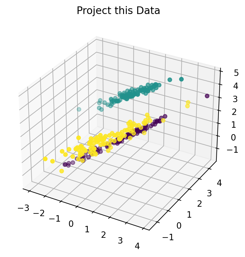
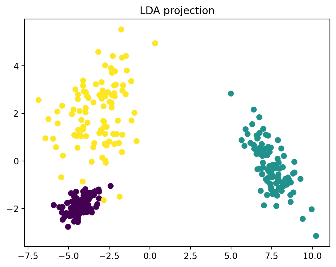
The effect of LDA or PCA is similar to seeing a 3D object with one eye: projection of higher dimension into one dimension.

LDA will use known class label.

Linear Discriminant Analysis (LDA) tries to identify attributes that account for the most variance between classes. In particular, LDA, in contrast to PCA, is a supervised method, using known class labels…

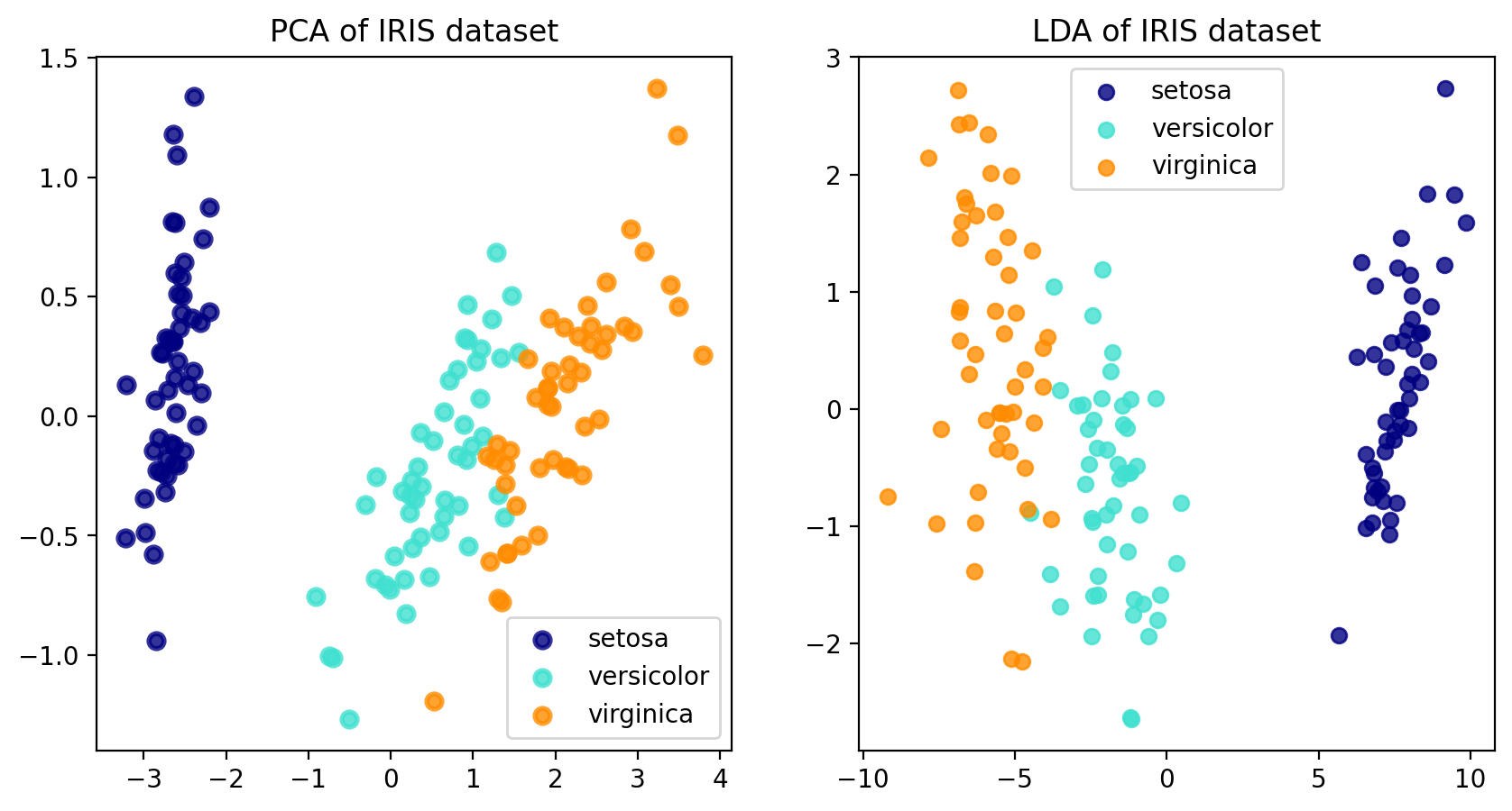
import matplotlib.pyplot as plt

from sklearn import datasets
from sklearn.decomposition import PCA
from sklearn.discriminant_analysis import LinearDiscriminantAnalysis

iris = datasets.load_iris()
X = iris.data
y = iris.target
target_names = iris.target_names

## fit model with principle component
pca = PCA(n_components=2)
X_r = pca.fit(X).transform(X)

## fit model with LDA
lda = LinearDiscriminantAnalysis(n_components=2)
X_r2 = lda.fit(X, y).transform(X)

## plog graph
fig, ax = plt.subplots(nrows=1,ncols=2,figsize=(10,5))
ax1=ax[0]
ax2=ax[1]

colors = ["navy", "turquoise", "darkorange"]
lw = 2

for color, i, target_name in zip(colors, [0, 1, 2], target_names):
    ax1.scatter(
        X_r[y == i, 0], X_r[y == i, 1], color=color, alpha=0.8, lw=lw, label=target_name
    )
ax1.legend(loc="best", shadow=False, scatterpoints=1)
ax1.set_title("PCA of IRIS dataset")


for color, i, target_name in zip(colors, [0, 1, 2], target_names):
    ax2.scatter(
        X_r2[y == i, 0], X_r2[y == i, 1], alpha=0.8, color=color, label=target_name
    )
ax2.legend(loc="best", shadow=False, scatterpoints=1)
ax2.set_title("LDA of IRIS dataset")

fig.show()

/var/folders/r5/1cdq52mn21zdnqzl0fvp44zw0000gn/T/ipykernel_98332/2715178903.py:43: UserWarning: Matplotlib is currently using module://matplotlib_inline.backend_inline, which is a non-GUI backend, so cannot show the figure.
  fig.show()

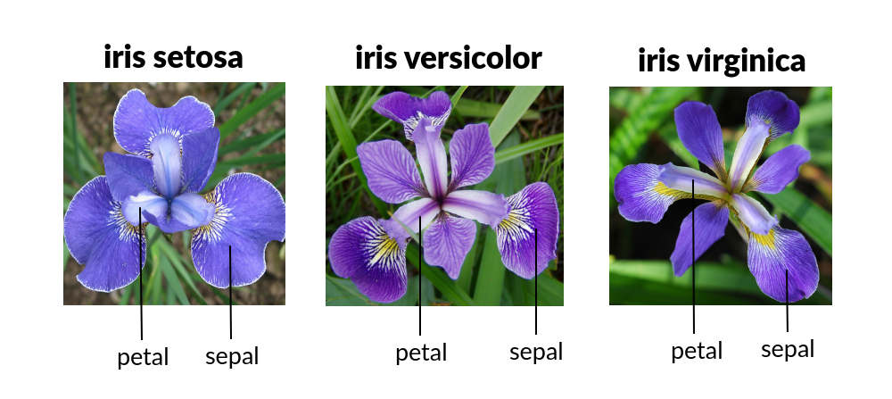
This following section it maybe useful for popup a few images of iris:

From an artist’s perspective the differences between these iris’s are dimensionality of petal and sepal. The latend varible here is probably can view as (how square are these two petal)

Detail LDA from Scratch

This blog post thanks to Andy Jones

import numpy as np
import matplotlib.pyplot as plt

# Generate data
mu1 = [0, 0]
mu2 = [1, 2]
cov = [[1, 0], [0, 1]]
n1 = 500
n2 = 50
n = n1 + n2
x1 = np.random.multivariate_normal(mean=mu1, cov=cov, size=n1)
x2 = np.random.multivariate_normal(mean=mu2, cov=cov, size=n2)
x = np.vstack([x1, x2])
y = np.concatenate([np.repeat(1, n1), np.repeat(2, n2)])


fig = plt.figure()
ax = fig.add_subplot()
ax.scatter(x[:, 0], x[:, 1], c=y)

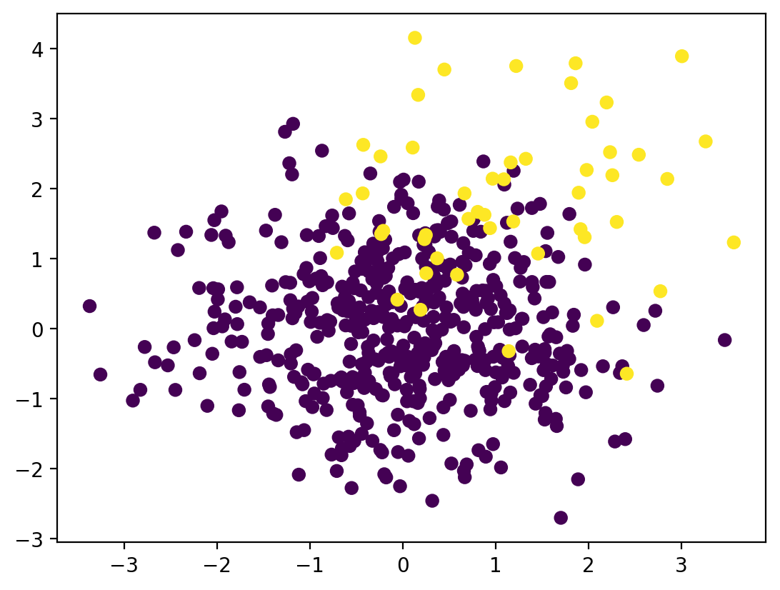
pi_hat_1 = n1 / n ## baysian prior also frequency of target
pi_hat_2 = n2 / n ## baysian prior also frequency of target

## avg,expected_value,or position of normal
mu_hat_1 = 1 / n1 * np.sum(x1, axis=0) #expected value for group1
mu_hat_2 = 1 / n2 * np.sum(x2, axis=0) #expected value for group2

# variance, or width of normal function
cov_hat_1 = 1 / (n1 - 1) * np.matmul((x1 - mu_hat_1).T, (x1 - mu_hat_1)) # with-in group co-variance
cov_hat_2 = 1 / (n2 - 1) * np.matmul((x2 - mu_hat_2).T, (x2 - mu_hat_2))
cov_hat = (cov_hat_1 + cov_hat_2) / 2

## defined log likelyhood function
def LL(x # any point pair
       , mu # average value
       , sigma # covariance
       , prior):
    dist = x - mu
    cov_inv = np.linalg.inv(sigma) ## inversion of cov matrix
    cov_det = np.linalg.det(sigma) ## determinant of cov matrix
    return -1/2 * np.log(2 * np.pi * cov_det) - 1/2 * dist.T @ cov_inv @ dist + np.log(prior)

## use this to test just so I simplify syntax of the function
# assert LL_(point_grid[0],mu_hat_1, cov_hat, pi_hat_1) == LL(point_grid[0],mu_hat_1, cov_hat, pi_hat_1)
## interestingly I also saw v.T * M * v.T in egen value + egen vector... so it reflect a common pattern of something? 
## `cov_inv @ dist` is actually 

Explain LL Formula:

In short LL is “Stacked Normal Distribution”

Given probability density function of a draw \(x_i\) from a normal distribute function:

\[ f(x_i; \mu,\sigma^2) = (2\pi\sigma^2)^\frac{1}{2}\exp(-\frac{1}{2}\frac{(x_i - \mu)^2}{\sigma^2}) \]

This function gives joint probability density function for give sample \(\xi=[x_1 ... x_n]\). This is the Likelihood Function

\[ \begin{align} L(\xi,\mu,\sigma^2) &= \prod_{i}^{n}{f(x_i; \mu,\sigma^2)} \\ &= (2\pi\sigma^2)^{-n/2}\exp(-\frac{1}{2\sigma^2} \sum_{i=1}^{n}{(x_i-\mu)^2} ) \end{align} \]

Because the area under density function is one, the joint probability function of varible would be many of these PDF stacked together. The mental image for this is think of any vector (no matter the sequence). The probability of \(\xi={x_1 ... x_n}\) occur follow above function and it doesn’t matter which order.

The Log-likelihood Function is just this function logged:

\[ \theta = (\mu;\sigma^2) \\ \begin{align} l(\theta; \xi) &= ln[(2\pi\sigma^2)^{-n/2}\exp(-\frac{1}{2\sigma^2} \sum_{i=1}^{n}{(x_i-\mu)^2} )] \\ &= ln[(2\pi\sigma^2) + \ln[exp(-\frac{1}{2\sigma^2} \sum_i^n{(x_i -\mu)^2} ))] \\ &= -\frac{n}{2}\ln(2\pi) - \frac{n}{2}\ln(\sigma^2) - \frac{1}{2\sigma^2}\sum_{i=1}^n{(x_i - \mu)^2} \end{align} \] The beauty of Log-Likelihood function is it canceled a lot of \(\exp\) element of normal distribution denity function and instead given you an algibratic expression, which you can then carry on to express with Matrix.

An Optimisation Problem

Log likelihoold function is used when \(\^{\theta}\) is unknown but a set of sample vector \(\xi\) is. This became a maximisation problem that obtain a \(\^{\theta}\) that will result that achieve this result. In the language of Math this is written as:

\[ \^{\theta} = \arg \max_{\theta}l(\theta; \xi) \]

(source: thanks to statlect)

Okay, now how LL is linked to LDA (Discriminant)?

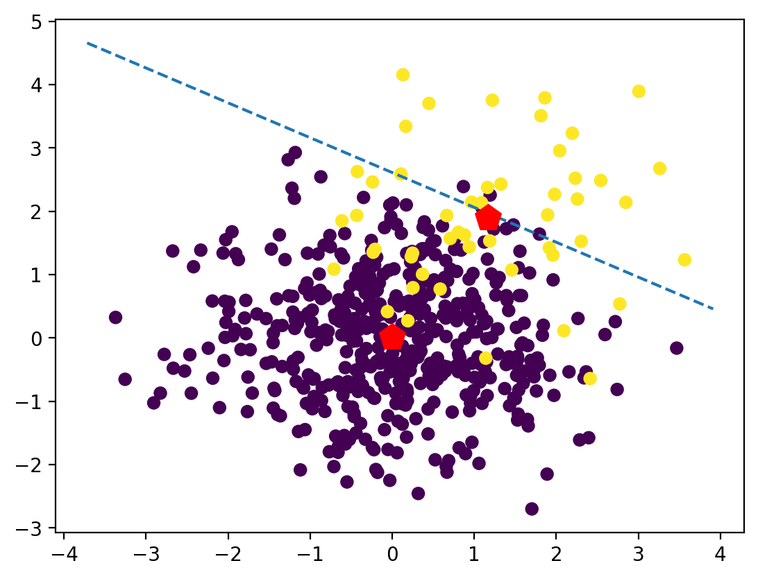
LDA approaches the problem by assuming that the condition \(p(x|y=0)\) and \(p(x|y=1)\) are both normal distribution, with mean and covariance parameter \((\mu, \sigma_0)\) \((\mu. \sigma_0)\), under this assumption, the Bayes-optimal solution is to predict points as being from the second class if the log of likelihood ratio is bigger than some threshold \(T\)

## I find it confusing when down to one dimension vector
## because NP consider it no difference vertical or horizontal
np.array([1,2]) @ np.array([[1,2],[3,4]]) ## so this is in fact consider first as horizontal
# 1 * 1 + 2 * 3 , 1 * 2 + 2 * 4
## this code below will result in different value
# np.array([[1,2],[3,4]]) @ np.array([1,2])

np.array([1,2]) @ np.array([[1,2],[3,4]]) @ np.array([1,2]) 
## 7 * 1  + 10 * 2

27

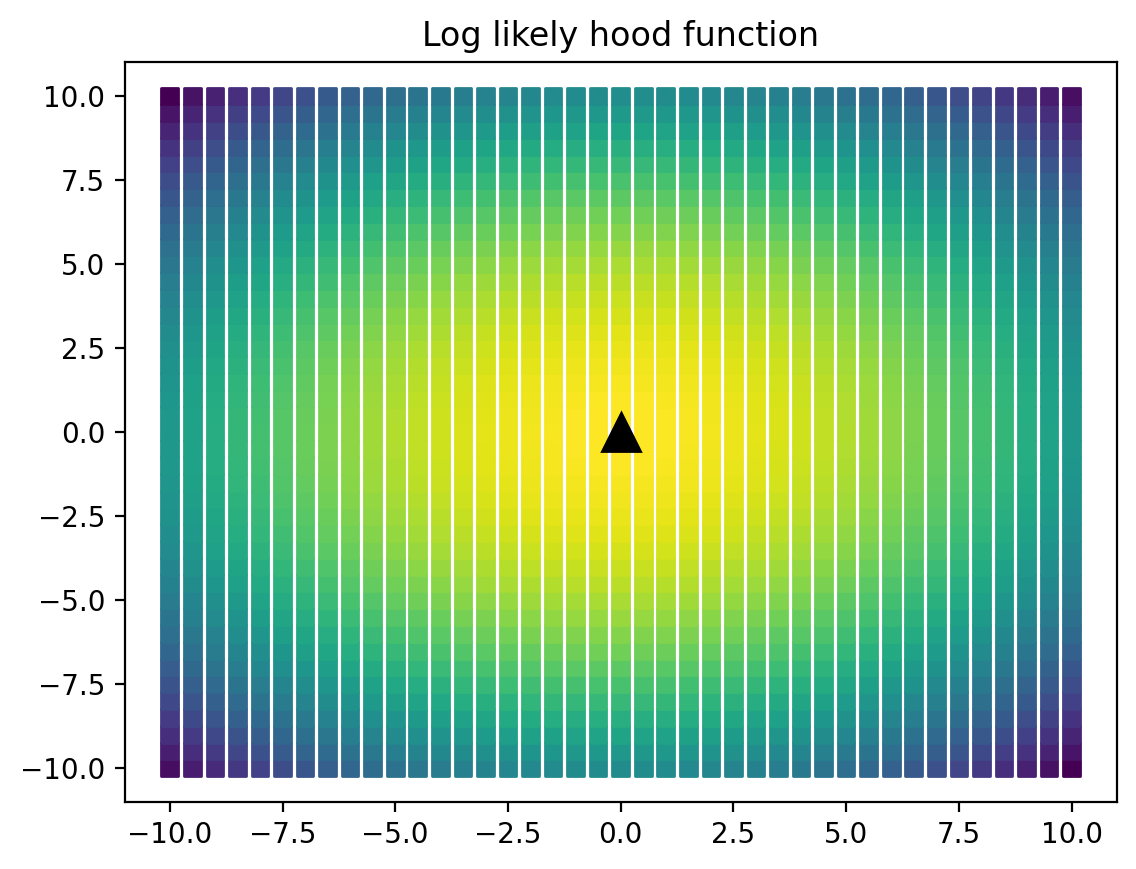
Display LL is a meshgird

point_grid = np.mgrid[-10:10.1:0.5, -10:10.1:0.5].reshape(2, -1).T
ll_vals_1 = [LL(x, mu_hat_1, cov_hat, pi_hat_1) for x in point_grid]
ll_vals_2 = [LL(x, mu_hat_2, cov_hat, pi_hat_2) for x in point_grid]


point_grid

fig = plt.figure()
ax = fig.add_subplot()

ax.scatter(point_grid[:, 0], point_grid[:, 1], c=ll_vals_1,marker="s")
ax.plot(mu_hat_1[0], mu_hat_1[1], 'k-^', markersize=14)
# ax.colorbar()
ax.set_title("Log likely hood function")

Text(0.5, 1.0, 'Log likely hood function')

cov_hat

array([[1.19308602, 0.01970993],
       [0.01970993, 1.0835684 ]])

def abline(slope, intercept):
    """Plot a line from slope and intercept"""
    axes = plt.gca()
    x_vals = np.array(axes.get_xlim())
    y_vals = intercept + slope * x_vals
    plt.plot(x_vals, y_vals, '--')
    
cov_inv = np.linalg.inv(cov_hat)

# slope
slope_vec = cov_inv @ (mu_hat_1 - mu_hat_2)
slope = -slope_vec[0] / slope_vec[1]

# intercept
intercept_partial = (
      np.log(pi_hat_2) - np.log(pi_hat_1) 
    + 0.5 * (mu_hat_1.T @ cov_inv @ mu_hat_1) 
    - 0.5 * (mu_hat_2.T @ cov_inv @ mu_hat_2))
intercept = intercept_partial / slope_vec[1]

# plotting
fig = plt.figure()
ax = fig.add_subplot()

ax.scatter(x[:, 0], x[:, 1], c=y)
abline(slope, intercept)
ax.plot(mu_hat_1[0], mu_hat_1[1], 'rp', markersize=14)
ax.plot(mu_hat_2[0], mu_hat_2[1], 'rp', markersize=14)

np.linalg.inv(cov_hat_1 + cov_hat_2) @ 

array([[ 0.41920724, -0.00762531],
       [-0.00762531,  0.46157704]])

Numpy Tips

mp.mgrid reshaping

# tip mash gird does this
np.mgrid[1:2.5:0.5, 1:2.5:0.5]# 

array([[[1. , 1. , 1. ],
        [1.5, 1.5, 1.5],
        [2. , 2. , 2. ]],

       [[1. , 1.5, 2. ],
        [1. , 1.5, 2. ],
        [1. , 1.5, 2. ]]])

np.mgrid[1:2.5:0.5, 1:2.5:0.5].reshape(2,-1).T

array([[1. , 1. ],
       [1. , 1.5],
       [1. , 2. ],
       [1.5, 1. ],
       [1.5, 1.5],
       [1.5, 2. ],
       [2. , 1. ],
       [2. , 1.5],
       [2. , 2. ]])