flat_matrix |>
  mutate(v=round(value, 2)) |>
  ggplot(aes(x,y)) +
  geom_tile(aes(fill=v)) +
  scale_fill_viridis_b(option = "G") +
  coord_equal()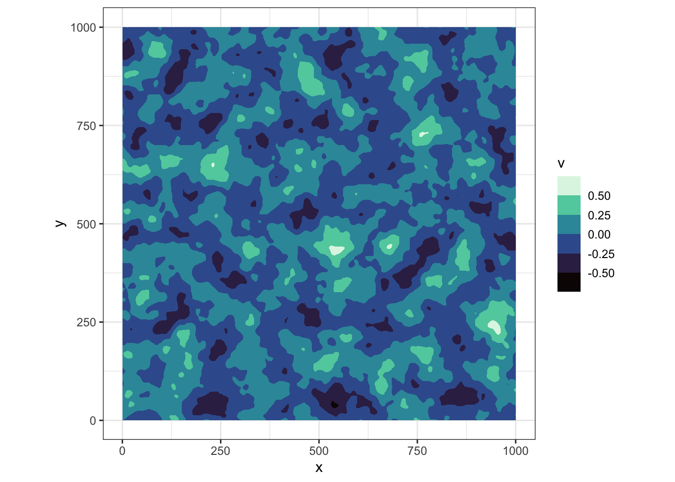
flat_matrix |>
mutate(v=round(value, 2)) |>
ggplot(aes(x,y)) +
geom_tile(aes(fill=v)) +
scale_fill_viridis_b(option = "G") +
coord_equal()
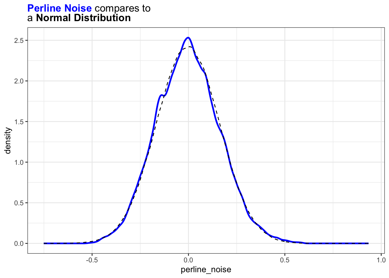
vs = sort(flat_matrix$value)
m = mean(vs)
sd = sd(vs)
rd = rnorm(length(vs), m,sd)

tibble(
  rank = 1:length(vs),
  perline_noise = vs,
  normal = rd |> sort()
) |>
  ggplot() +
  geom_density(aes(x = perline_noise),color="blue",linewidth=1) +
  geom_density(aes(x = normal),linetype="dashed") +
  ggtitle(
    glue::glue("<span style='color: blue'><b>Perline Noise</b></span> compares to <br>"
               ,"a <b>Normal Distribution</b>")
  ) +
  theme(
    title = ggtext::element_markdown()
  )
rec = c(xmin = 50, xmax = 100, ymin = 50, ymax = 100)

flat_matrix |>
  mutate(v=round(value, 2)) |>
  ggplot(aes(x,y)) +
  geom_tile(aes(fill=v)) +
  scale_fill_viridis_b(option = "G") +
  coord_equal() +
  annotate("rect", xmin=50,xmax=100,ymin=50,ymax=100,fill=NA,color="green")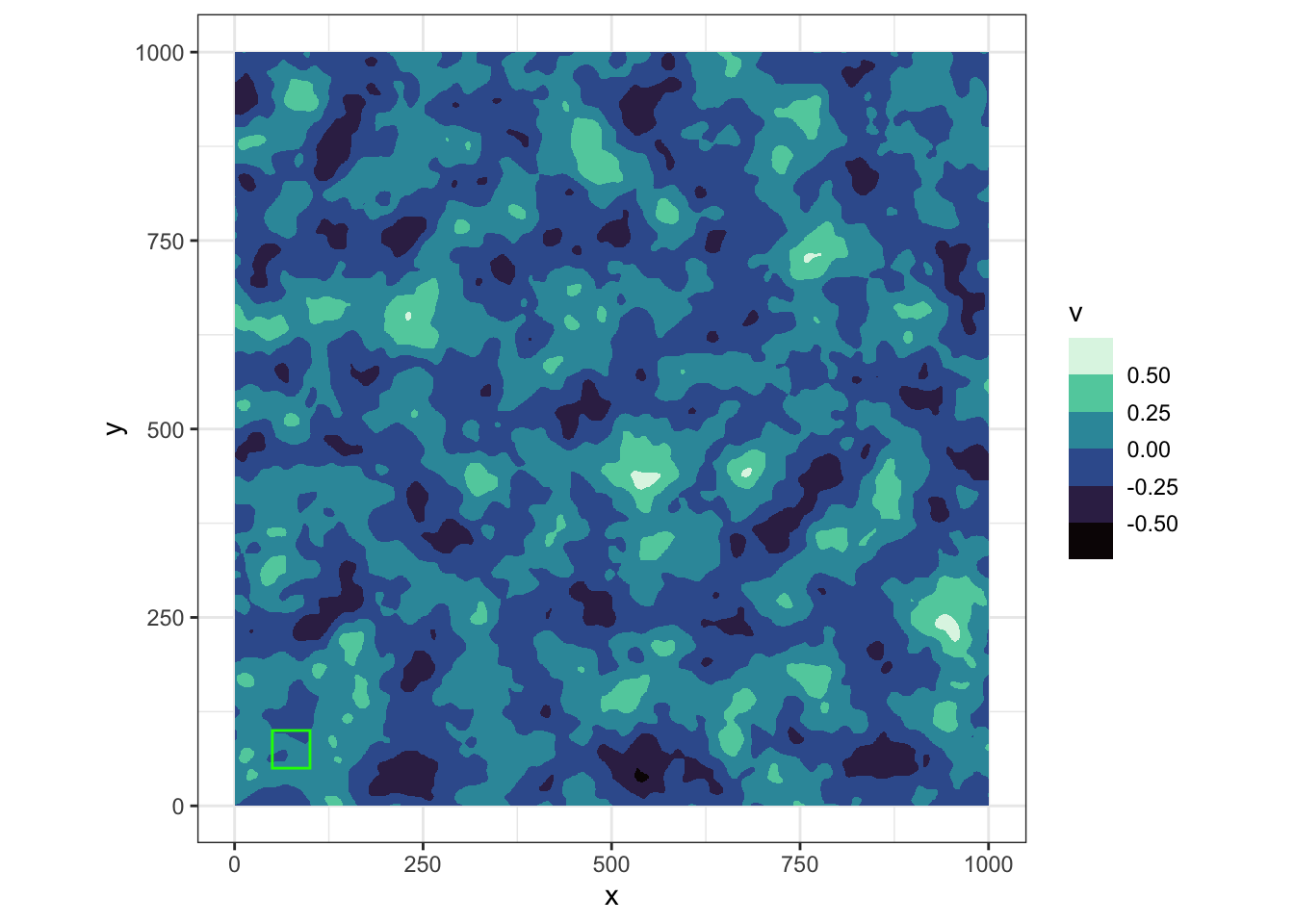
Experiment with a small square of data
## select a small sample
flat_matrix |>
  filter(x |> between(rec["xmin"], rec["xmax"]) & y |> between(rec["ymin"], rec["ymax"])) |>
  mutate(v=round(value, 2)) |>
  ggplot(aes(x,y)) +
  geom_tile(aes(fill=v)) +
  scale_fill_viridis_b(option = "G") +
  coord_equal()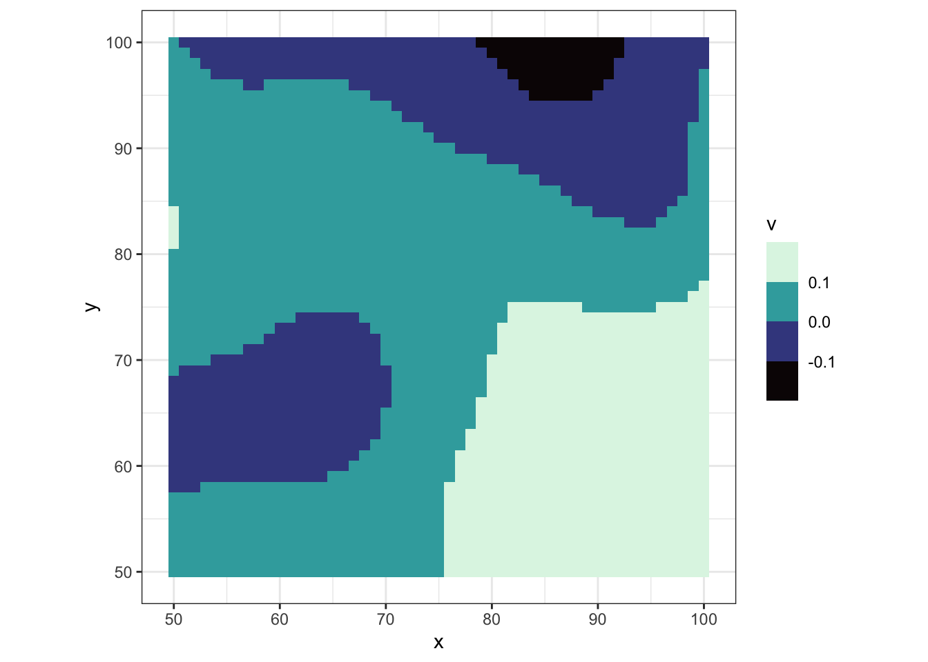
res=5
init_angle = 0.01 * 2 * pi #10% of a circle which is 36°

flat_matrix |>
  ## sample a few point
  filter(x |> between(rec["xmin"], rec["xmax"]) & y |> between(rec["ymin"], rec["ymax"])) |>
  filter(x %%res ==0 & y %% res == 0) |>

  ## make a vector points
  mutate(
    stv = diff(c(min(value),value)) / diff(range(value)),
    angle = stv * 2 * pi,
    d = res * 0.66,
    x_p = sin(angle + init_angle) * d + x,
    y_p = cos(angle + init_angle) * d + y
  ) |>

  mutate(v=round(value, 2)) |>
  ggplot(aes(x,y)) +
  geom_segment(aes(x=x,xend=x_p,y=y,yend=y_p),arrow=arrow(length = unit(0.1,"inches")),alpha=0.7) +
  geom_point(aes(color=v),alpha=0.33) +
  geom_point(aes(x=x_p, y_p,color=v),alpha=1) +
  scale_color_viridis_b(option = "G") +
  coord_equal()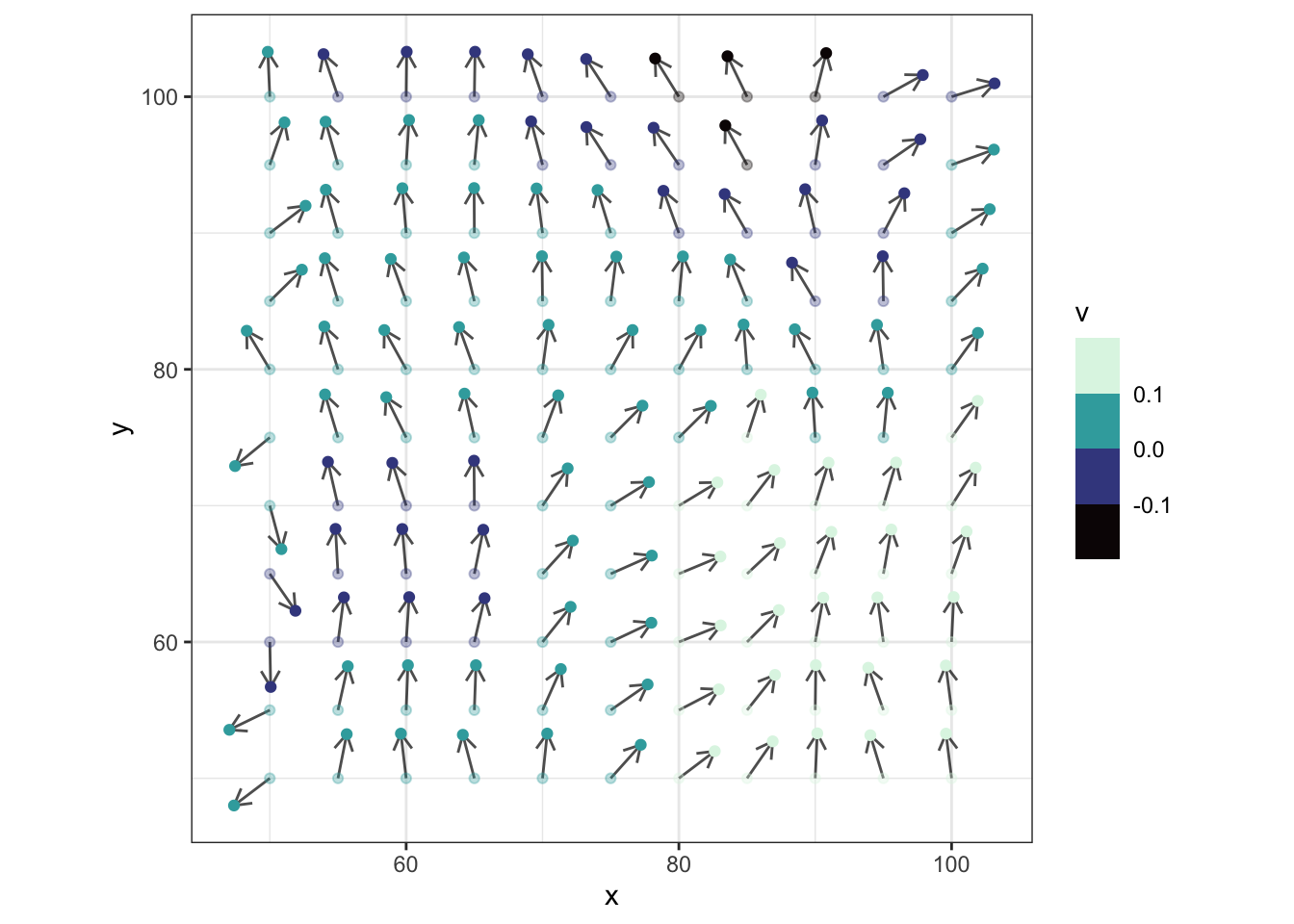
make_rect = function(x=200, y=200, d = 400) {
  return( c(xmin = x - d/2, xmax = x + d/2, ymin = y - d/2, ymax = y + d/2))
}
annotate_rect = function(rec,...) {
  return(list(annotate("rect"
                       , xmin=rec['xmin']
                       , xmax=rec['xmax']
                       , ymin=rec['ymin']
                       , ymax=rec['ymax']
                       , fill = NA
                       , ...)))
}
crop = function(data, rec = make_rect()) {
  data |>
  ## sample a few point
    filter(x |> between(rec["xmin"], rec["xmax"]) & y |> between(rec["ymin"], rec["ymax"]))
}
de_res = function(data, res = 15) {
  data |>
    filter(x %%res ==0 & y %% res == 0)
}
val_to_angle = function(data,value,init_angle = 0.01 * 2 * pi) {
  data |>
    mutate(
      angle = {{value}} * 2 * pi + init_angle,
    )
}
res = 15
angle_matrix = flat_matrix |>
## sample a few point
val_to_angle(value)
g_grid = angle_matrix |>
de_res(res=res) |>
crop() |>
## make a vector points
mutate(
d = res * 0.6,
x_p = cos(angle ) * d + x,
y_p = sin(angle ) * d + y
) |>
mutate(v=round(value, 2)) |>
ggplot(aes(x,y)) +
geom_segment(aes(x=x,xend=x_p,y=y,yend=y_p),arrow=arrow(length = unit(0.02,"inches")),alpha=0.7) +
scale_color_viridis_b(option = "G") +
coord_equal()
g_grid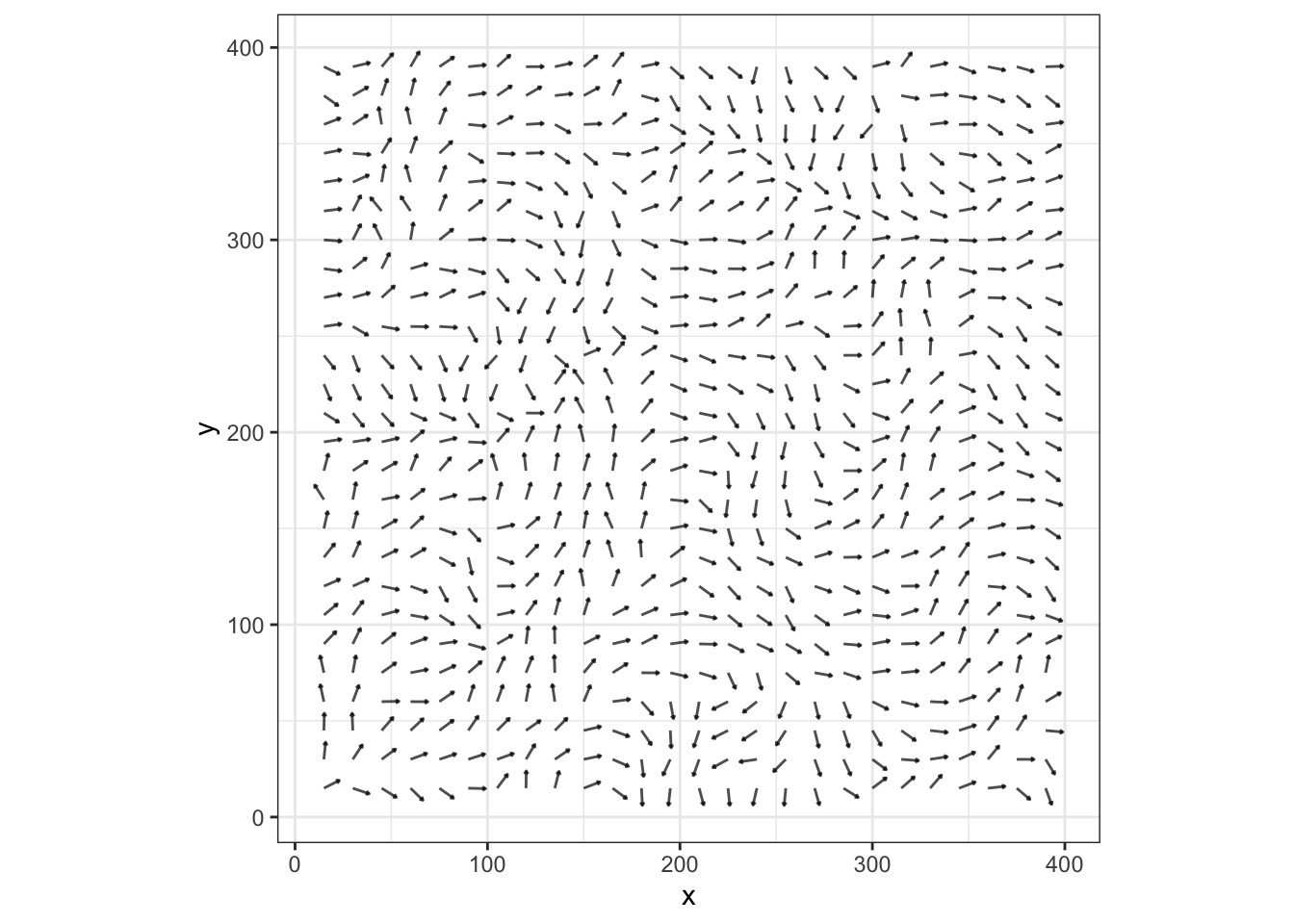
Nice! Next try release particle to the data grid:
This is very simple in this grid system because we simply just round to neast point?
sample_rec = make_rect(100,300,100)

t_angle_matrix = angle_matrix |>
  # de_res(res=res) |>
  crop()

## Set a Group Parameter
seed_particle = t_angle_matrix |>
  crop(sample_rec) |>
  slice_sample(n=16) |>
  mutate(.group = row_number(), id=0)

particles_path = seed_particle
particle = seed_particle

### A Simple Find My Particle graph
for (i in 1:500) {
  next_coord = particle |>
    mutate(
        x = x + round(cos(angle))
      , y = round(y + sin(angle))
      , id = i
      ) |>
    select(id,x,y,.group)
  particle = t_angle_matrix |>
    inner_join(next_coord,c("x","y"))
  if(nrow(particle) == 0) {
    break
  }
  particles_path = particles_path |> bind_rows(particle)
}

# particle_smooth = smooth.spline(particles_path)
g_grid +
  geom_path(
    data = particles_path |>
      mutate(xx=x,yy=y),
     # mutate(xx=particle_smooth$x, tt=particle_smooth$y),
    aes(x = xx, y = yy,group=.group),color="#4c16fb",size=0.7,
    # stat="smooth"
  ) +
  # facet_wrap(~.group) +
  annotate_rect(sample_rec,color="#2ecc71",alpha=0.5,linewidth=0.8) +
  ggtitle(
    "",
    subtitle=glue::glue(
      "Random <span style='color:#4c16fb'><b>partical path</b></span> samped from <br>the ",
      "<span style ='color:#2ecc71' ><b>green rectangle</b></span>"
      )
  ) +
  theme(
    title=ggtext::element_markdown()
  )
Warning: Using `size` aesthetic for lines was deprecated in ggplot2 3.4.0.
ℹ Please use `linewidth` instead.
Something poetic about this system. Imagine the dotes are people, vectors are social tendencies, influence of our parent’s, influence of the school teacher.
we are all born on this green square but different people scattered up to different places yet fate draw them to one place.
[tbc]