Thank you EARL 2026
8th October, I gave a light-hearted lighting talk titled “let’s hunt alien” EARL 2026, in Brighton! For those of you who was with us and enjoyed by talk, a big thank you! I’m overwhelmed by your reactions. And thank you to Data Cove team, specfically Laura who has given me so much encouragement.
The talk is based on my blog back in Jun 2024 , so most of the code will be there!
Side note, I wanted this talk to be a almost a scifi movie watching experience so I styled the last slide like a movie credit scene.
Additional Code
Most code will be in my original code blog back in Jun 2024 . The only other code missing here is clustering and wrangling.
Load relevant datas
library (dplyr)library (dbplyr)library (ggplot2)library (duckdb)## So the only way is to laod that data from geometry <- DBI:: dbConnect (duckdb:: duckdb ("ufo.db" ,read_only = TRUE ))= conn |> tbl ("analysis.ufo_observe_by_state_year" )= conn |> tbl (sql ("select * exclude geometry, st_asWkB(geometry) as geometry from clean.us_state_polygon" ))= conn |> tbl (sql ("from clean.us_population" )) |> group_by (county_id) |> slice_max (n= 1 ,order_by= api_year) |> select (county_id,fullname= GEONAME) |> collect () |> # this is to make the name in a printable format for visualise on specific state mutate (full_name= stringr:: str_extract (fullname, "[ \\ w \\ s]+,[ \\ w \\ s]+" ) |> :: str_replace (", \\ s" ," \n " )|> collect ()= ufo_data |> left_join (us_counties, "county_id" ) |> mutate (year = as.integer (year))class (mart) <- c ("ufo_mart" ,class (mart))
My favourite way of doing this in R is to create a S3 class for different dataframe.
Functions To Help with Aggregation & Graphics
= function (df) {|> summarise (ufo_count = sum (ufo_count),ufo_multi_observe = sum (ufo_multi_observe),geometry = first (geometry),density = mean (as.numeric (DENSITY), na.rm= TRUE ),population = mean (as.numeric (POP))|> mutate (ufo_count_density = (ufo_count / density),ufo_multiserve_density = (ufo_multi_observe / density)= function (df) {= df |> collect () |> mutate (geometry= sf:: st_as_sfc (geometry, crs= 4269 )|> :: st_as_sf ()class (x) <- c ("ufo_mart" , class (x))return (x)= function (df, variable, ..., title) {|> :: tm_shape () + :: tm_polygons (fill = variable,fill.scale = tmap:: tm_scale_continuous_pseudo_log (fill.legend = tmap:: tm_legend (position= c ("right" ,"bottom" ),title= title),+ :: tm_layout (legend.outside= TRUE )= function (x) {if (inherits (x, "ufo_mart" )) {return (x)else {class (x) <- c ("ufo_mart" , class (c))return (x)= function (...) {UseMethod ("vis" )}= function (...) {UseMethod ("collect_sf" )}= function (...) {UseMethod ("agg" )}= function (...){as_ufo_mart (NextMethod ("mutate" ))= function (...) {UseMethod ("vis_top_score" )}= function (x, desc= TRUE , label_from = "full_name" , colorpalette = "brewer.bu_pu" , text_size= 0.7 ,limits= c ()= enquo (variable)= as_label (variable)if (length (limits) == 0 ) {= pull (x, {{variable}}) |> range ()= x |> arrange ({{variable}} |> desc ())if (desc) {= x |> slice_head (n= top_n)else {= x |> slice_tail (n= top_n)= pull (x, {{variable}}) |> median ()= glue:: glue ("{{{label_from}}}" )|> # transform mutate ("{var_label}" : = round (!! variable,2 ),text_color= ifelse ({{variable}} > mid_point, "white" , "black" ),label = glue:: glue (label_glue)|> :: st_as_sf () |> :: tm_shape () + :: tm_polygons (fill= var_label,fill.scale = tmap:: tm_scale_continuous_log (values= colorpalette),fill.legend = tmap:: tm_legend_hide (),fill_alpha= 0.5 ,limits= limits+ :: tm_text (text= "label" ,col= "text_color" ,size= text_size
Function wraper for spdep local moran
# Local Moran Statistics ----------------------- = function (variable, nb, get = c ("Ii" ,"E.Ii" ,"Var.Ii" ,"Pr(z > E(Ii))" )) {= spdep:: nb2listw (nb, style= "W" ,zero.policy = TRUE )= spdep:: localmoran_perm ( {{variable}}, lw, alternative= "greater" )= function (variable, nb, get = c ("Ii" ,"E.Ii" ,"Var.Ii" ,"Pr(z > E(Ii))" )) {= spdep:: nb2listw (nb, style= "W" ,zero.policy = TRUE )= spdep:: localmoran_perm ( {{variable}}, lw, alternative= "greater" )attributes (t)$ quadr$ mean
# some interesting event data = sf:: st_point (c (- 115.80833 ,37.23333 )) |> :: st_sfc (crs= 4326 )= sf:: st_point (c (- 71.05 ,42.36 )) |> :: st_sfc (crs= 4326 )= mart |> filter (year > 1890 ) |> group_by (county_id) |> agg () |> collect_sf ()= spdep:: poly2nb (ufo_state_summary_since_xxxx, queen= TRUE )= ufo_state_summary_since_xxxx |> mutate (ufo_density_moran_p = local_moran_c (ufo_count_density,nb, "Pr(z > E(Ii))" ),ufo_density_moran_i = local_moran_c (ufo_count_density,nb,"Ii" ),ufo_density_lisa = local_moran_c_quadr (ufo_count_density,nb)|> left_join (tibble:: as_tibble (us_count_full_name_) |> select (county_id, full_name) )
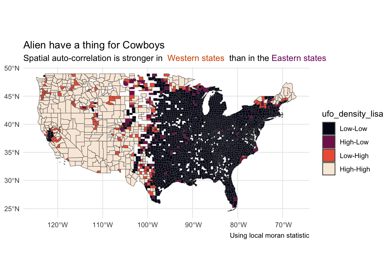
Local Moran’s I Map
|> ggplot () + geom_sf (aes (geometry= geometry, fill= ufo_density_lisa)+ scale_fill_viridis_d (option = "F" ) + theme_minimal () + theme (plot.title = ggtext:: element_markdown (),plot.subtitle = ggtext:: element_markdown (),plot.caption = ggtext:: element_markdown ()+ labs (title= "<span style='font-weight: bold'>Alien have a thing for Cowboys</span>" ,subtitle= "Spatial auto-correlation is stronger in <span style='color: #D35400 font-weight: bold'> Western states </span> than in the <span style='color: #7C0969'>Eastern states</span>" ,caption= "Using local moran statistic"
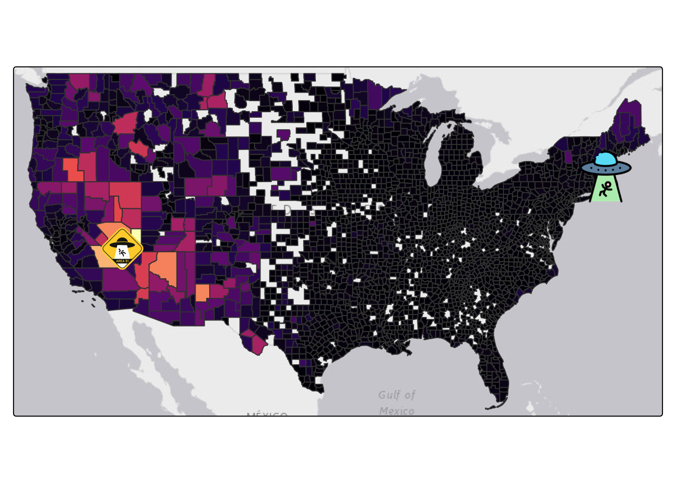
UFO Sighting Absorbed Population Density
|> DBI:: dbExecute ("load spatial;" )= conn |> tbl (sql ("select * from clean.ufo_data_standardized" )) |> collect () |> mutate (geometry = sf:: st_as_sfc (geometry,crs= 'EPSG:4269' )|> :: st_as_sf ()
Observation Heatmap with annotation
ℹ tmap modes "plot" - "view"
ℹ toggle with `tmap::ttm()`
Observation Heatmap with annotation
= "black" = "#F5B027" = "#28B463" = "magma" ## scatter plot mini map --------------------- = ufo_state_summary_since_xxxx |> # left_join(us_count_full_name_, by="county_id") |> arrange (ufo_density_moran_i |> desc ()) |> mutate (label = full_name) |> head (2 )= top_x_county |> :: st_as_sf () |> :: tm_shape () + :: tm_basemap () + :: tm_polygons () + :: tm_text (text= "label" ,col= "white" ,size= 0.5 = ufo_points |> inner_join (select (tibble:: as_tibble (top_x_county), county_id), by= "county_id" ) |> :: tm_shape () + :: tm_symbols (shape = tmap:: tmap_icons ("asset/ufo.png" ),size= 0.3 = tmap:: tm_shape (dot_area_51) + :: tm_symbols (shape= tmap:: tmap_icons ("asset/Area-51-UFO-Sign.png" ),## Another minimap for visualise first UFO sighting event = tmap:: tm_shape (dot_massachuesetts_bay) + :: tm_symbols (shape = tmap:: tmap_icons ("asset/alien-abduction.png" )## big choro plot mini map --------------------- # tmap::tmap_mode("plot") |> :: tm_shape () + :: tm_basemap () + :: tm_polygons (id = "county_id" ,fill = "ufo_count_density" ,fill.scale = tmap:: tm_scale_continuous_pseudo_log (values= .moran_color_fill,fill.legend = tmap:: tm_legend_hide ()+ :: tm_layout (legend.outside= TRUE ) + + :: tm_text (text= "51" ,col= "white" ,size = 0.7 +
UFO Sighting without Absorbed Population Density
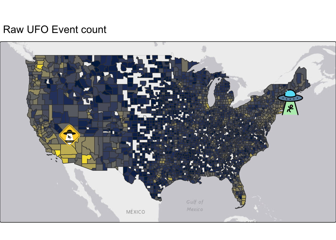
Raw UFO count without anything
ℹ tmap modes "plot" - "view"
Raw UFO count without anything
= ufo_state_summary_since_xxxx |> slice_max (ufo_count) |> mutate (text = glue:: glue (" {round(ufo_count)} Alien Sighting in {full_name} " )) |> :: tm_shape () + :: tm_polygons (fill= "midnightblue" ) + :: tm_text (text= "text" ,col= "white" )|> :: tm_shape () + :: tm_basemap () + :: tm_polygons (fill = "ufo_count" ,fill.scale = tmap:: tm_scale_continuous_pseudo_log (values= 'cividis' ,fill.legend = tmap:: tm_legend_hide ()+ + + # tmap::tm_inset(top_count,group_id = "1",height=20, width = 20, position = c("right","bottom")) + # tmap::tm_components(group_id = "1", position = c("bottom","left")) + :: tm_layout (legend.outside= TRUE ,outer.margins = rep (0 ,4 ),inner.margins = rep (0.09 ,4 )+ :: tm_title ("Raw UFO Event count" )